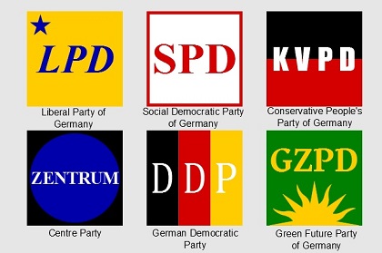
Popular german political parties
There are essentially 3 datasets,train_df, election_results_german_federal_states_df and federal_elections_germany_survey_df. We then drop the columns with too much null values and too little variance in data.
# dropping columns with little variance in data

from sklearn.feature_selection import VarianceThreshold
var_thres_train=VarianceThreshold(threshold=0)
var_thres_election=VarianceThreshold(threshold=0)
var_thres_federal=VarianceThreshold(threshold=0)

var_thres_train.fit(train_df_mod[["result","turnout","dimap_pred","FGW_pred"]])

var_thres_election.fit(election_results_german_federal_states_df_mod[["CDU","SPD","Die Gruenen","FDP","Die Linke","AfD"]])

var_thres_federal.fit(federal_elections_germany_survey_df_mod[["CDU","SPD","GRÜNE","FDP","LINKE","AfD","Sonstige"]])
Afterwards, we convert the train_df to a datetime time-series and observe the change of popularity in the different political parties. We also look at the time series of the SPD, CDU and GRÜNE party.
For federal elections and surveys, we observe that CDU, SPD and GRÜNE are the 3 most popular candidates. We then create a scatterplot to observe the frequency of CDU pollings in the last 12 years.

Popular german political parties